Pump Performance in PI Vision for Water/Utilities
Using the PI Asset Framework and Aveva PI Vision displays to monitor and gain visibility into Pump Performance.
Introduction
We recently finished a project to develop a pump performance monitoring solution based on PI Asset Framework elements and PI Vision displays. Getting insight into a pump’s performance can be challenging as the performance can only be calculated based on the environment, and the performance curves are in 3-dimensional space: flow, head, and rotation speed.
The pump performance is usually monitored in a spreadsheet, which seems to be a convenient way to develop the solution. However, it has multiple drawbacks, even if they appear at the beginning. These drawbacks include the basic issues with spreadsheets regarding distribution and updating, as well as more specific issues with time-series data regarding how to update the current values or the historical time ranges.
In this solution, we managed to use the PI Asset Framework‘s templating power to model and describe the environment of the pumps, the built-in tables and lookup attributes to store pump curve data, and PI Vision to visualize the pump curves. The PI system’s centralized nature helps us with distribution and updates, while the PI Vision’s natural way of displaying time-series data fixes the issue of displaying data updates.

The pump curves
Pump curves are tabular data that represent the pump performance.
The data includes flow, speed, head, power, and efficiency.
In our case, the pump curve data has been stored in books, so we get it in scanned PDF format. The data was provided with the handover of the pumps years ago, so gathering this included traditional data mining on bookshelves. We added this data into the PI Tables, including IDs, and made-up datetime values to mimic that time-series data. The dates are on a specific date, and each line has a different time for that day. This trick will enable us to draw the pump curves on the PI Vision displays that are designed to show time series data. Later, we will see how.
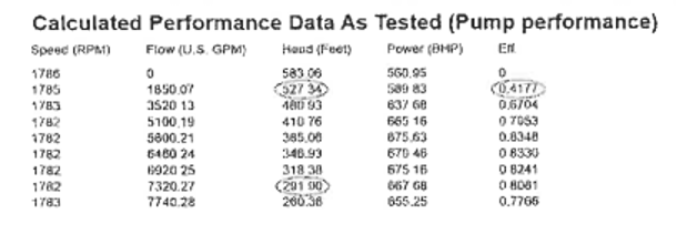
We also added information about the system curve. The system curve describes how the resistance of the pipes and tanks upstream from the pumps (the system) changes with different flow rates. So, this is a head–flow rate table. Engineers usually calculate this information. We also received this data in a spreadsheet format and added it the same way we did with the pump curves.
The tables created were then turned into a time-series data source in the PI Asset Framework. The values are separated into multiple speed regimes, so each pump speed from the document has its individual AF attribute. This is done by the table lookup data reference, where the head, power, and efficiency are selected as the result, the speed is a filter value, and the made-up datetime values are the timestamps.
Measured Values
After gathering the theoretical values, we should also calculate the actual measured values that we want to plot next to the pump curves.
Flow
In this specific case, pumps didn’t have separate flow measurements. The flow is measured at the pump station level and divided by the pump running signal. This way, we can get an individual calculated flow that can be plotted on the screen. This is created with PI Analysis using both expressions and rollups.
Head
The head is the energy that the pumps give to the pumped water. It is described by how high the pump can deliver the liquid and is expressed in feet or meters. The height or head is used because the pump generates the same head and different pressure with different liquids. The head can describe the pump agnostic to the transported liquid.
The conversion between pressures and elevation can described by Bernoulli’s principle as it is described in this drawing:
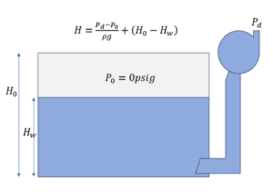
This calculation can be easily templated and calculated with PI Analysis expressions.
Power
Power is usually calculated already on control system level. If it isn’t then it can be calculated based on electrical potential and current measurements. Also we have to take into account the electric motors efficiency, that can be considered constant in most cases.
Efficiency
This efficiency is the efficiency of the pump, so we have to monitor how the pump turns the rotation coming from the motor into liquid flow.

The pump power (Ppump) is the power we just calculated in the previous chapter.
hydraulic power (Phydraulic) is more complex, but we can reuse some already existing calculations. Power is how fast we can move mass from one point to another. This translates in case of pumps that how much mass flowrate can we transport for a given head. So, we just have to multiply the flow rate the density and the head and we receive the hydraulic power we are looking for.
This is how we can calculate the necessary values that can be plotted against the theoretical pump curve values
PI Vision Displays
The previous steps helped to calculate the values, but we also had to show them in meaningful format.
Presenting the measured values can be done in PI Vision out of the box; however, there is a limit to the number of samples that can be shown on the screen. To handle this, we created two separate displays where you can change the sample rate: one with a one-minute sample rate for more details and another with a one-hour sample rate for longer time ranges. We added links to easily switch between these screens.
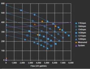
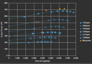
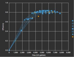
We also had to add the pump curve plots. These plots are not time series data but curves that don’t change as time passes. Fortunately, there is an option to fix the time displayed for a specific plot, as we set the displayed time range to the made-up datetime values that we introduced when the pump curve data was entered into the PI system. Selecting that we also want to connect the samples will result in a nice curve for each rotation speed.
Summary
As you can see, we could store the pump curve data in PI that was earlier in books. We could calculate the different operating parameters that best describe the pump’s performance. In PI Vision, we could create displays that can make the comparison of theoretical and measured values easy. This would enable the operation team to easily identify the different kinds of mechanical and leakage problems or to monitor the performance of the pump stations.
Are you interested in learning more about how IT Vizion’s PI Vision and Aveva PI System Services coupled with our domain expertise can help you make sense of your data? Contact us to schedule a conversation.

IT Vizion is the OT/IT system integrator of choice for some of the largest Oil&Gas, Chemicals, and Manufacturing companies worldwide.
Copyright ©2026 IT Vizion
Contact info
Let’s connect. Contact IT Vizion today.
- We Operate Worldwide
- +1 (951) 256-4320
- [email protected]
